According to 老板,according to yifan,这本书很好,所以我就来学习一下了。
Part 1 的说明
Measuring Performance
Changing a seemingly unrelated part of the source code can surprise us with a significant impact on program performance. This phenomenon is called measurement bias. … Instead, we will just focus on high-level ideas and directions to follow.
This chapter will give a brief introduction to why modern systems yield noisy performance measurements and what you can do about it.
Noise In Modern Systems
一种叫 Dynamic Frequency Scaling 的技术可以短时间内提升 CPU 的频率,但它是基于核心温度的,所以不确定。在散热不太好的笔记本上经常发生第一个 run 会 turbo,但第二个 run 回归到 base frequency 的情况。
软件层面的因素,包括 file cache 是否 warm。有论文说,env var 的大小,以及 link 的顺序都能影响性能。影响内存布局也可以影响性能,有研究说 efficiently and repeatedly randomizing the placement of code, stack, and heap objects at runtime 可以解决处理内存布局带来的问题。
如果 benchmark 一个云处理器环境,上述的 noise 和 variation 基本难以被消除。
temci 这个工具能够设置环境,从而确保一个 low variance。
Measuring Performance In Production
CPU Microarchitecture
Instruction Set Architecture
the critical CPU architecture and microarchitecture features that impact performance
In addition to providing the basic functions in the ISA such as
load, store, control, scalar arithmetic operations using integers and floating-point, the widely deployed architectures continue to enhance their ISA to support new computing paradigms. These include enhanced vector processing instructions (e.g., Intel AVX2, AVX512, ARM SVE) and matrix/tensor instructions (Intel AMX). Software mapped to use these advanced instructions typically provide orders of magnitude improvement in performance.
深度学习中,即使使用较少的 bits 效果也挺好,所以一些处理器倾向于引入 8bit integer 等来节约计算和内存带宽。
Pipelining
The processing of instructions is divided into stages. The stages operate in parallel, working on different parts of different instructions.
在 CSAPP 里面已经学习了取指、解码、执行、访存、写回的流水线。
The throughput of a pipelined CPU is defined as the number of instructions that complete and exit the pipeline per unit of time.
The latency for any given instruction is the total time through all the stages of the pipeline.
The time required to move an instruction from one stage to the other defines the basic machine cycle or clock for the CPU. The value chosen for the clock for a given pipeline is defined by the slowest stage of the pipeline. 因此这里的优化点是均衡或者重新设计 pipeline,消除最慢的 stage 的 bottleneck。
假定所有的 stage 都是完美 balanced,没有任何 stall,那么通过 pipeline,可以让一个指令的处理时间减少到原来的 n_stage 分之一。
下面提到三种冒险,其中 Structural hazard 指的是对硬件资源的争抢,通常通过复制硬件解决。剩下两种在 CSAPP 中详细介绍过了,本教程做了归纳。
数据冒险是程序中的数据依赖,分三类:
Read after write
x 的写结束前,x + 1 就需要读到 x 的写的内容,不然 x + 1 会读到更旧的数据。通常使用 bypassing 的办法,将数据从流水线的后面(指令 x + 1 的阶段) forward 到前面(指令 x 的阶段)。Write after read
x 在读完之后,x + 1 才能写,不然 x 会读到更新的数据。译码阶段总是在写回阶段前面,为什么会有 WAR 场景?原因是需要考虑处理器乱序执行。如下所示,R0 上存在 WAR 场景。1
2R1 = R0 ADD 1
R0 = R2 ADD 2WAR 可以被 register renaming 解决。 Logical (architectural) registers, the ones that are defined by the ISA, are just aliases over a wider register file。因此,只需要将第二个 R0,以及之后的所有的 R0 重命名到另一个寄存器文件上即可解决问题。因此这两个指令之间就可以被乱序执行了。
【Q】这些 physical register file 如何被 gc 呢?旧的 R0 alias 不知道新的 R0 alias 的存在啊。看 CPU backend 的介绍时发现,这个是 ROB 做的。Write after write
同样可以通过 register renaming 解决。
控制冒险主要指分支预测之类的东西,影响取指阶段。诸如动态分支预测、 speculative execution 能优化。
Exploiting Instruction Level Parallelism (ILP)
大多数的指令可以被并行执行,因为它们是不相关的。
OOO Execution
An instruction is called retired when it is finally executed, and its results are correct and visible in the architectural state. To ensure correctness, CPUs must retire all instructions in the program order. 这里 architectural state 主要区分于 microarchitectural state,后者是隐藏的 state,例如 pipeline registers、cache tag、branch predictor 等。
OOO is primarily used to avoid underutilization of CPU resources due to stalls caused by dependencies, especially in superscalar engines described in the next section.
scoreboard 被用来 schedule the in-order retirement and all machine state updates。它需要记录每一条指令的数据依赖 and where in the pipe the data is available。scoreboard 的大小决定了 CPU 能够超前多少调度彼此无关的指令。
下图中,x + 1 因为一些冲突,插入了一些气泡。而 OOO 的执行可以使 x + 2 这个 independent 的指令先进入执行(EXE)阶段。但是所有的指令还是要 按照 program order 来 retire,也就是最后的写回阶段是要按顺序的。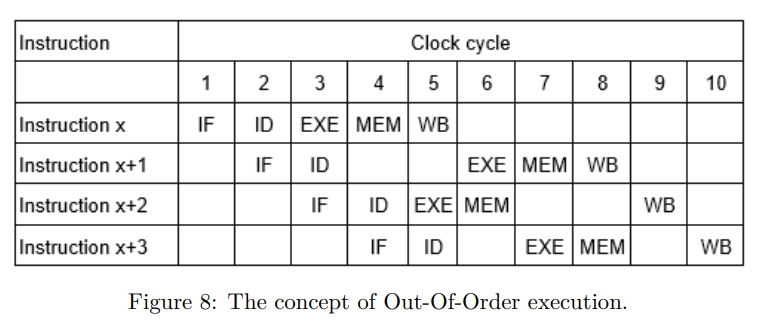
Superscalar Engines and VLIW
Most modern CPUs are superscalar i.e., they can issue more than one instruction in a given cycle. Issue-width is the maximum number of instructions that can be issued during the same cycle.
目前处理器的 issue width 在 2 到 6 之间。为了处理这些 instruction,目前 CPU 也会支持 more than one execution unit and/or pipelined execution units。Superscalar 也可以和之前提到的 pipeline 和 OOO 结合起来用。
下图展示了 issue width = 2 的情况。 Superscalar CPU 中支持多个 independent execution units 能够执行指令,而避免冲突。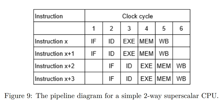
Intel 使用 VLIW,即 Very Long Instruction Word 技术将调度 Superscalar 和 multi execution unit 的负担转移给编译器。这是因为 software pipelining, loop unrolling 这些编译器优化相比硬件能看到的更多。
Speculative Execution
下面介绍了 Speculative Execution 是什么,不翻译了。
As noted in the previous section, control hazards can cause significant performance loss in a pipeline if instructions are stalled until the branch condition is resolved. One technique to avoid this performance loss is hardware branch prediction logic to predict the likely direction of branches and allow executing instructions from the predicted path (speculative execution).
如下所示,Speculative Execution 不会等 branch 预测结果,而是直接执行 foo,如打星号所示,但是实际的状态变化直到 condition 被 resolve 之后才会被 commit,这样才能保证 architecture state 不会被 speculative executing 影响。
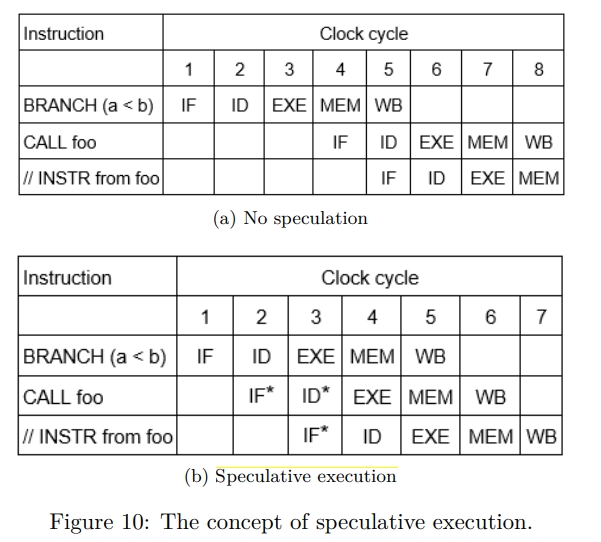
在现实中,branch 命令可能依赖从内存中加载上来的某个值,这可能需要花费上百个 cycle。如果分支预测的是不正确的,也就是实际应该调用 bar 了,那么 speculative 执行的结果需要被扔掉,称为 branch misprediction penalty。
为了记录 speculation 的进度,CPU 支持一个叫 ReOrder Buffer 即 ROB 的结构。ROB 中依照顺序了所有指令,包括已经 retire 的指令的状态。如果 speculation 是正确的华,speculative execution 的结果按照 program order 会写到 ROB 里面,然后被 commit 到 architecture register 中。
CPUs can also combine speculative execution with out-of-order execution and use the ROB to track both speculation and out-of-order execution.
Exploiting Thread Level Parallelism
A hardware multi-threaded CPU supports dedicated hardware resources to track the state (aka context) of each thread independently.
The main motivation for such a multi-threaded CPU is to switch from one context to another with the smallest latency (without incurring the cost of saving and restoring thread context) when a thread is blocked due to a long latency activity such as memory references
Simultaneous Multithreading
ILP techniques and multi-threading 被结合使用。不同线程中的指令在同一个 cycle 中被并发地执行。同时从多个线程中 dispatch 指令可以充分利用 superscalar 资源,提高 CPU 总体性能。为了支持 SMT,CPU 需要复制硬件去存储 thread state,例如 PC 和寄存器等。追踪 OOO 和 speculative execution 的资源可以复制,也可以共享。一些 Cache 被 hardware 线程共享。
Memory Hierarchy
Memory Hierarchy 从下面两种性质构造:
- Temporal locality
- Spatial locality
CSAPP 中进行了更为详细的讨论。
Cache Hierarchy
A particular level of the cache hierarchy can be used exclusively for code (instruction cache, i-cache) or for data (data cache, d-cache), or shared between code and data (unified cache).
Placement of data within the cache
Finding data in the cache
Managing misses
对 direct-mapped 来讲,它会 evict 掉之前的 block。
对 set-associative 来讲,需要一个例如 LRU cache 的算法。
Managing writes
CPU designs use two basic mechanisms to handle writes that hit in the cache:
- In a write-through cache
hit data is written to both the block in the cache and to the next lower level of the hierarchy - In a write-back cache
hit data is only written to the cache.
Subsequently, lower levels of the hierarchy contain stale data.
The state of the modified line is tracked through a dirty bit in the tag. When a modified cache line is eventually evicted from the cache, a write-back operation forces the data to be written back to the next lower level.
Cache misses on write operations can be handled using two different options:
- write-allocate or fetch on write miss cache
数据会被从下一级缓存中被加载上来,并且当前 write operation 会被视作一次 write hit。 - no-write-allocate policy
cache miss 会直接被发送到下一级缓存,并且该缓存不会被加载到当前缓存。
Out of these options, most designs typically choose to implement a write-back cache with a write-allocate policy as both of these techniques try to convert subsequent write transactions into cache-hits, without additional traffic to the lower levels of the hierarchy.
Write through caches typically use the no-write-allocate policy.
Other cache optimization techniques
1 | Average Access Latency = Hit Time + Miss Rate × Miss Penalty |
硬件工程师们努力减少 Hit Time,以及 Miss Penalty。而 Miss Rate 取决于 block size 和 associativity,以及软件。
HW and SW Prefetching
Prefetch 指令和数据可以减少 cache miss 和后续的 stall 的发生。
Hardware prefetchers observe the behavior of a running application and initiate prefetching on repetitive patterns of cache misses. Hardware prefetching can automatically adapt to the dynamic behavior of the application, such as varying data sets, and does not require support from an optimizing compiler or profiling support. Also, the hardware prefetching works without the overhead of additional address-generation and prefetch instructions. 当然,hardware prefetching 只限于某几种 cache miss pattern。
Software memory prefetching 中,开发者可制定一些内存位置,或者让编译器自行添加一些 prefetch 指令。
Main memory
Main memory uses DRAM (dynamic RAM) technology that supports large capacities at reasonable cost points.
主存被三个属性描述,latency、bandwidth 和 capacity。
Latency 主要是两个指标,Memory access time 是从请求,到数据 available 的时间。Memory cycle time 是两个连续的访存操作之间最小的时间间隔。
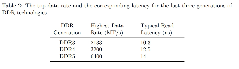
DDR (double data rate) DRAM 是主要的 DRAM 技术。历史上,DRAM bandwidth 每一代都会被提高,但是 DRAM 的 latency 原地踏步,甚至会更高。下面的表中展示了最近三代的 DDR 技术的相关数据。MT/s 指的是 a million transfers per sec。
Virtual Memory
Virtual Memory 实现多个程序共享一个内存。具有特性:
- protection
也就是不能访问其他进程的内存 - relocation
也就是不改变逻辑地址,但是将程序加载到任意的物理地址
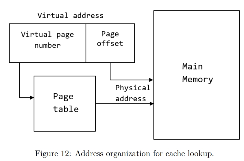
vitual 地址和物理地址通过 page table 进行转换。vitual 地址分为两部分。virtual page number 用来索引具体的 page table,这个 page table 可能是一层,也有可能嵌套了很多层。page offset 用来 access the physical memory location at the same offset in the mapped physical page。
如果需要的 page 不在主存里面,就会发生 page fault。操作系统负责告诉硬件去处理 page fault,这样一个 LRU 的 page 会被 evict 掉,腾出空间给新 page。
CPUs typically use a hierarchical page table format to map virtual address bits efficiently to
the available physical memory. CPU 会使用一个有层级的 page table 去维护 virtual address 和 physical memory 的关系。但 page fault 的惩罚是很大的,需要从 hierarchy 中 traverse 查找。所以 CPU 支持一个硬件结构 translation lookaside buffer (TLB) 来保存最近的地址翻译结果。
SIMD Multiprocessors
SIMD (Single Instruction, Multiple Data) multiprocessors 是相对于之前的 MIMD 来说的。SIMD 会在一个 cycle 中将一条指令运用于多个数据上,从而利用多个 functional units。
下图是 SISD 和 SIMD 的对比。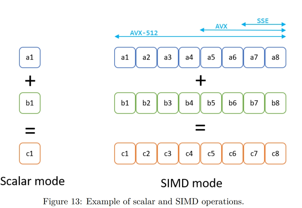
Modern CPU design
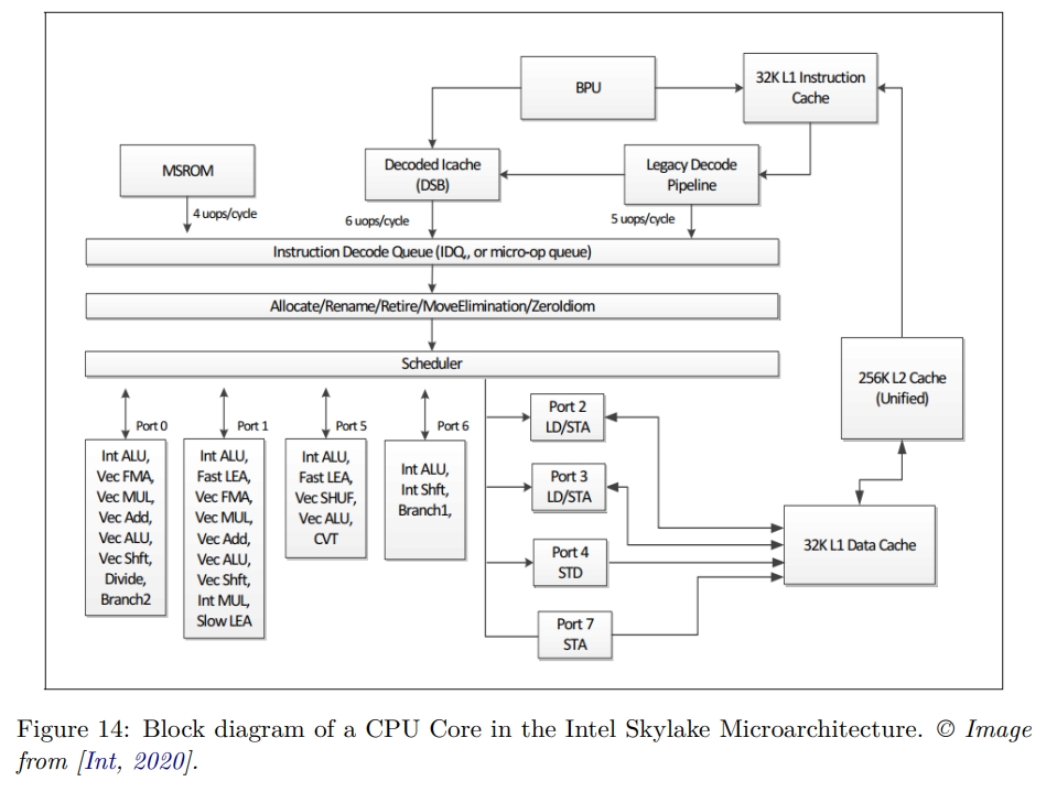
下图是 Skylake(2015) 的架构。 The Skylake core is split into an in-order front-end that fetches and decodes x86 instructions into u-ops and an 8-way superscalar, out-of-order backend.
The core supports 2-way SMT. It has a 32KB, 8-way first-level instruction cache (L1 I-cache), and a 32KB, 8-way first-level data cache (L1 D-cache). The L1 caches are backed up by a unified 1MB second-level cache, the L2 cache. The L1 and L2 caches are private to each core.
CPU Front-End
前端负责 fetch and decode instructions from memory,将准备好的指令喂给后端执行。
每一个 cycle,前端从 L1 I-cache 中取 16 bytes 的指令。它们被两个线程分享,所以实际上是第一个周期线程 A 取,第二个周期线程 B 取,然后又是线程 A 这样。这些指令是复杂的可变长度的指令,pipeline 的 pre-decode 和 decode 阶段将它们分成 micro Ops(UOPs),并且把它们排在 Allocation Queue (IDQ) 队列中。
pre-decode 主要标记指令的边界。指令的长度从 1 到 15 bytes 不等。这个阶段还 identifies branch instructions。这个阶段移动最多 6 条指令,或者称为 Macro Instructions 到 instruction queue 中。instruction queue is split between the two threads. instruction queue 中有个 macro-op fusion unit,可以检测两个 macroinstructions 是否可以 fuse 为一个指令、
一个周期中,最多5个被 pre-decode 完毕的指令会被发送到 instruction queue,同样是两个线程轮流分享这个接口。Decoder 将复杂的 macro-Op 转化为固定长度的 UOP,也就是上文提到的 micro Op。Decoder 是 5-way 的。
前端主要的性能提升组件是 Decoded Stream Buffer (DSB),或者称为 UOP Cache。它的目的是将 macro Op 到 UOP 的转换保存在单独的 DSB 结构中。在取指阶段,会先在 DSB 查询。频繁执行的 macro op 会命中 DSB,pipeline 就能够避免昂贵的 pre-decode 和 decode 环节。
DSB 提供 6 个 UOP,这个和前端到后端的接口匹配。DSB 和 BPU 也就是 branch prediction unit 协同工作。
一些非常复杂的指令需要超过 decoder 能够处理的 UOP,它们就会被送给 Microcode Sequencer (MSROM) 处理。这些命令包含字符串处理、加密、同步等指令。另外,MSROM 也会保存 microcode operation,以便处理分支预测出错(需要刷新 pipeline),或者 floating-point 等异常情况。
Instruction Decode Queue (IDQ) 是在 inorder 的前端和 OOO 的后端之间的桥梁。每个 hardware thread 上 IDQ 大小 64 个 UOP,总计大小 128 UOP。
CPU Back-End
后端是一些 OOO engine,执行指令并且存储结果。
后端的心脏是一个 ReOrder Buffer,即 ROB,它有 224 条 entry。它的功能:
- 维护 architecture-visible registers 到 physical registers 的映射。这个映射被 Reservation Station/Scheduler (RS) 使用。
- 支持 register renaming。
- 记录 speculative execution。
ROB entry 按照 program order retire。
Reservation Station/Scheduler (RS) 结构记录一个 UOP 所使用的所有资源的 availablility。一旦这些资源满足了,就会将这个 UOP dispatch 到某一个 port。因为 the core(不知道指的是什么)是 8-way superscalar,所以 RS 在一个 cycle 中可以 dispatch 最多 8 个 UOP。如上面图 14 所示,这些 Port 分别支持不同的操作:
- Ports 0, 1, 5, and 6 provide all the integer, FP, and vector ALU. UOPs dispatched to those ports do not require memory operations.
- Ports 2 and 3 are used for address generation and for load operations.
- Port 4 is used for store operations.
- Port 7 is used for address generation.
Performance Monitoring Unit
Performance Monitoring Counters
这也就是后面在 Sampling 中提到的 PMC。PMC 会收集 CPU 中各个组件的统计信息。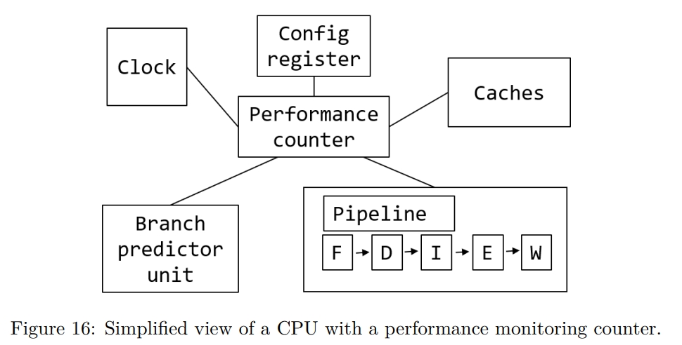
一般来说,PMC 有 48bit 宽,这样可以允许分析工具能够跑更长时间,而不至于被中断触发。这是因为当 PMC overflow 的时候,程序执行会被中断,SW 需要存储 overflow 的情况。在 Sampling 章节也会进一步看到分析工具是如何利用这个特性的。
PMC 是 HW register,被实现为 Model Specific Register(MSR)。也就是具体有哪些,每种 CPU 是不一样的,并且 width 也不一定是 48bit。
Terminology and metrics in performance analysis
perf 命令或者 Intel VTune Profiler 里面的术语很难懂,本章进行介绍。
Retired vs. Executed Instruction
- 正常情况,the CPU commits results once they are available, and all precedinginstructions are already retired.
- Speculative 执行,the CPU keeps their results without immediately committing their results. When the speculation turns out to be correct, the CPU unblocks such instructions and proceeds as normal. 如果预测失败,则会丢弃所有的结果,并且不 retire 它们。
CPU Utilization
CPU 不在跑 idle 线程的时候,即被认为是 utilize 的。
CPI & IPC
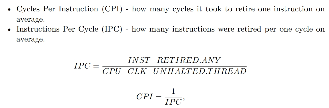
UOPs (micro-ops)
Microprocessors with the x86 architecture translate complex CISC-like instructions into simple RISC-like59 microoperations - abbreviated µops or uops. 这里 CISC 指的是 Complex Instruction Set Computer。RISC 指的是 Reduced Instruction Set Computer。
这个转换的好处在于,UOP 可以被 OOO 地执行。一个简单的加法指令,例如 ADD EXA,EBX 只会产生一个 UOP。而一个复杂的指令,例如 ADD EAX,[MEM1] 可能生成两个 UOP,一个用来读内存到一个临时的,没有名字的寄存器中,另一个指令将这个临时寄存器中的数字加到 EAX 中。同理,ADD [MEM1],EAX 会产生三个 UOP,一个读内存,一个加,一个写内存。不同的 CPU 处理这些指令,比如如何将它们划分为不同的 UOP 的方式,是不一样的。
除了将复杂的 CISC-like 的指令分解为 RISC-lick 的 UOP 或者说 microoperations 之外,还有一种策略是融合一些指令。有两种融合的类型:
Microfusion
对同一个指令中的多个 UOP 进行 fuse。如下所示,访存操作和加法在 decode 阶段被 fuse 了。1
2
3# Read the memory location [ESI] and add it to EAX
# Two uops are fused into one at the decoding step.
add eax, [esi]Macrofusion
如下所示,一个代数计算和一个条件跳转指令被 fuse 为一个 compute-and-branch UOP 了。1
2
3
4# Two uops from DEC and JNZ instructions are fused into one
.loop:
dec rdi
jnz .loop
Both Micro- and Macrofusion save bandwidth in all stages of the pipeline from decoding to retirement. The fused operations share a single entry in the reorder buffer (ROB). The capacity of the ROB is increased when a fused uop uses only one entry。我想这就是为什么要 fuse 指令的原因,因为它们节约了 ROB 的空间。在执行的时候,这个表示两个操作的 ROB entry 会被两个 execution units 处理,被发送到两个不同的 execution ports,但最后作为一个 unit 被 retire。
Linux perf users can collect the number of issued, executed, and retired uops for their workload by running the following command:
1 | $ perf stat -e uops_issued.any,uops_executed.thread,uops_retired.all -- a.exe |
Pipeline Slot
A pipeline slot represents hardware resources needed to process one uop.
Core vs. Reference Cycles
Reference Cycles 是 CPU 计算 cycle 数量,仿佛没有 frequency scaling 一般。相当于不 tuebo,base frequency 下运行的 cycles。
1 | $ perf stat -e cycles,ref-cycles ./a.exe |
The core clock cycle counter is very useful when testing which version of a piece of code is fastest because you can avoid the problem that the clock frequency goes up and down.
Cache miss
Mispredicted branch
1 | $ perf stat -e branches,branch-misses -- a.exe |
Performance Analysis Approaches
Code Instrumentation
比如用 printf 调试,打印一个函数执行了多少次这样。这是 macro level 的,而不是 mirco level 的。
这个技术的主要用处是,能够快速定位到具体问题的模块。因为性能问题不仅和代码有关,也和数据有关。例如一个场景渲染比较慢,有可能是数据压缩问题,也有可能是场景元素过多。
当然,缺点就是只在 app 层级,到不了内核以及更下层。另外,调试代码需要重新编译,会降低性能,甚至改变现场。
Binary instrumentation 技术的特点:
- 对二进制分析
- 提供 static 和 dynamic 两种模式
dynamic 模式可以动态开启,可以限制只对某些函数调试
诸如 Intel Pin 的工具可以拦截某个事件,并且在之后插入代码。
- instruction count and function call counts.
- intercepting function calls and execution of any instruction in an application.
- allows “record and replay” the program region by capturing the memory and HW registers state at the beginning of the region.
Tracing
strace 工具跟踪系统调用,可以被视作对内核的测量。Intel Processor Traces 工具跟踪 CPU 指令,可以被视作对 CPU 的测量。
Tracing is often used as the black-box approach, where a user cannot modify the code of the application, yet they want insight on what the program is doing behind the scenes。
Tracing 用来检查异常。例如一个系统十秒都不响应了,这个时候,Code Instrumentation 可能就不管用,但 tracing 可以去了解到底发生了什么。
Workload Characterization
Workload characterization is a process of describing a workload by means of quantitative parameters and functions。
Counting Performance Events
用一个 Counter 记录在跑一个 workload 时,某个事件在一段时间内发生的次数。
Manual performance counters collection
一般来说,不建议直接观察 PMC,而是使用 Intel Vtune Profiler 去看一个处理后的结果。
可以通过 perf list 查看可以访问的 PMC。
1 | $ perf list |
对于没列出的,可以使用下面的来检查
1 | perf stat -e cpu/event=0xc4,umask=0x0,name=BR_INST_RETIRED.ALL_BRANCHES/ |
Multiplexing and scaling events
考虑到有时候需要同时记录多个事件,但只有一个 counter。所以 PMU 会为每个 HW 线程提供四个 counter。但可能还是不够。
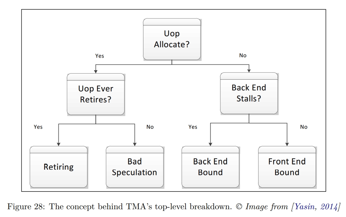
Top-Down Analysis Methodology (TMA) 需要一次执行过程中收集最多 100 个不同的 performance event。
这个时候,就引入了 multiplexing 技术,如下图所示。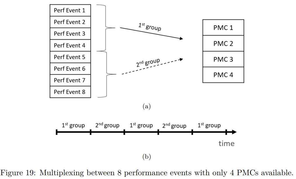
Sampling
人们常常用 profiling 这个词去指代 sampling,但其实 profiling 这个词包含的范围更广。
User-Mode And Hardware Event-based Sampling
User-mode sampling 是个 SW 方案,也就是在用户程序中 embed 一个库。这个库会为每个线程设置 OS timer,在 timer 超时的时候,程序会收到 SIGPROF 信号。
EBS 是一个 HW 方案,它使用 PMC 去触发中断。
SW 方案只能被用来发现热点。而 HW 方案还可以被用来采样 cache miss,TMA(section 6.1) 等。
SW 方案的 overhead 更大。HW 方案更准确,因为允许采样更多的数据。
Finding Hotspots
下面的一个技术使用了 counter overflow 技术。也就是当 counter 溢出的时候,触发 performance monitoring interrupt(PMI)。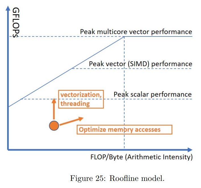
我们不一定要 sample CPU cycle,例如如果要检查程序中哪里出现了最多的 L3 cache miss,就可以 sample MEM_LOAD_RETIRED.L3_MISS 这个事件。
流程如下:
- 配置 PMC 去计算某项指标,例如 cycle 数
- 在执行过程中,PMC 会递增
- PMC 最终会 overflow,HW 会触发 PMI
- Profile 工具会抓住中断,并使用配置了的 Interrupt Service Routine(ISR) 去处理这个事件
- 禁止掉 counting
- reset counter 到 N
- 继续 benchmark 过程
通过 N 的不同取值,可以决定采样的频率。
Collecting Call Stacks
常见情况是,最热点的函数是被多个 caller 调用的。这个时候就需要知道是 Control Flow Graph (CFG) 里面的哪一条路径导致的。想要去追踪 foo 的所有 caller 是很耗时的,但我们只是想最终那些导致 foo 变成 hotspot 的,或者说是想找到 CFG 中经过 foo 的最热的路径。
下面三种方法:
- Frame pointer
perf record –call-graph fp
这需要二进制被以 -fnoomit-frame-pointer 形式编译。历史上,Frame pointer 也就是 BP 寄存器被用来 debug,是因为它允许 get the call stack without popping all the arguments from the stack(stack unwinding)。Frame pointer 可以直接告诉我们 return address。 - DWARF debug info
perf record –call-graph dwarf
这需要程序被按照 -g (-gline-tables-only) 形式编译。 - Intel Last Branch Record (LBR)
perf record –call-graph lbr
这种方式得到的 call graph 的深度不如前面两者。
Flame graph
相比上面提到的,一个更流行的办法是火焰图。
Roofline Performance Model
这里的 roofline 指的是应用程序的性能不会超过机器本身的容量。每个函数或者每个循环都会被机器本身的计算或者内存容量所限制。
HW 有两方面限制:
- 它可以算多快
FLOPS - 它可以多快传输数据
GB/s
一个程序的不同部分,会有不同的 performance characteristics。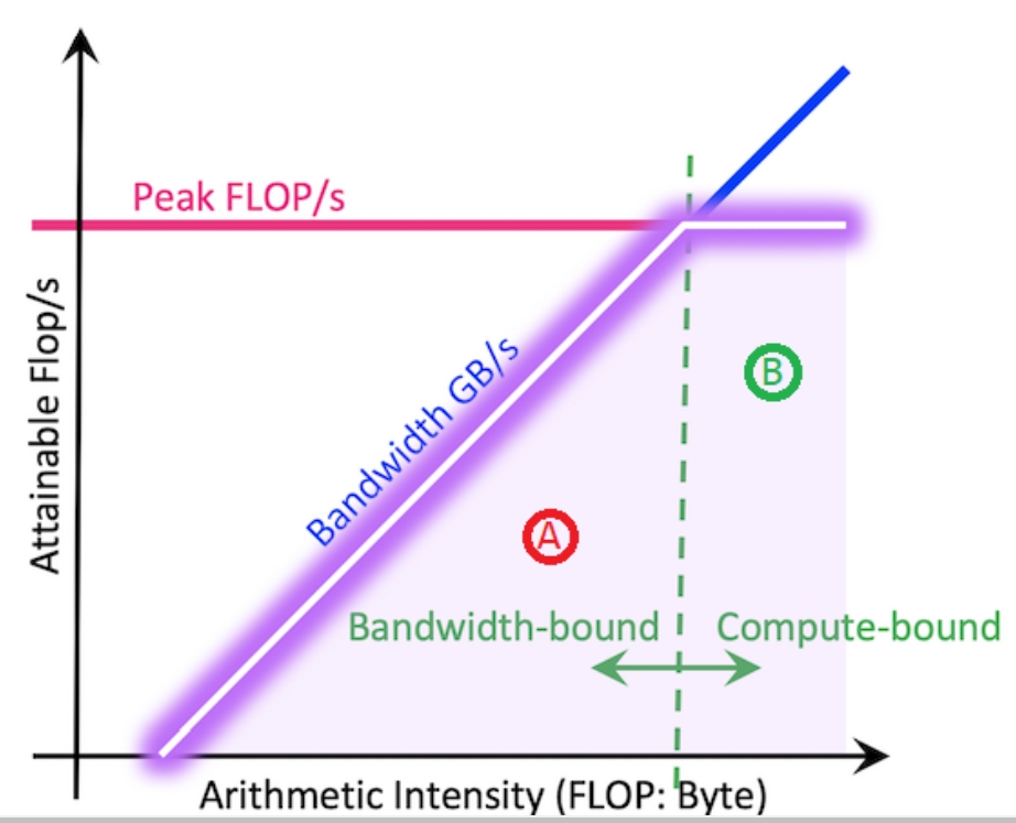
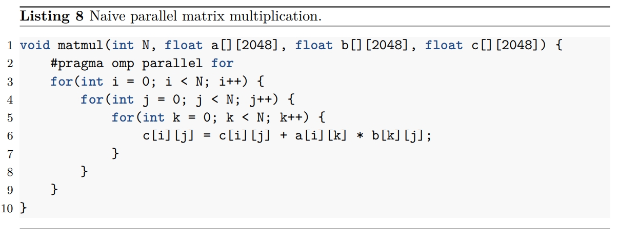
Arithmetic Intensity (AI) is a ratio between FLOPS and bytes and can be extracted for every loop in a program。不妨对下面的代码来算一下。在最内层循环有一个加法和一个乘法,所以是 2FLOPS。另外,还有三个读操作和一个写操作,所以传输了 4 * 4 = 16 字节。所以 AI 是 2 / 16 = 0.125。这作为图表的横轴。
一般来说,提高程序性能可以分为 vectorization、memory、threading 三个方面。Roofline methodology 可以帮助评估应用的特征。如下所示,在 roofline 图表上,我们可以画出单核、SIMD 单核和 SIMD 多核的性能。因此可以借助于图表来判断优化方向。AI 越高,说明越是 CPU bound 的,就越要考虑 CPU 方面的优化。Vectorization 和 threading 的操作一般能够让图表中的点上移,而 optimize memory access 的操作一般能够将点右移,也可能能将点上移。
Roffline 分析可以进行前后的对比,如下所示,在执行完交换内外循环,以及 vectorize 后,性能发生了提高。
Static Performance Analysis
Compiler Optimization Reports
CPU Features For Performance Analysis
通常来说,profiling 能够快速发现应用程序的 hotspots。例如考虑 profile 一个函数,你觉得它应该是 cold 的,但你发现它实际花了很长时间并且被调用了很多次。所以你可以使用 cache 等技术来减少调用的次数,从而提高性能。
当主要的性能优化点都被处理后,就需要 CPU的支持来发现新的性能瓶颈了。所以在了解本章之前,需要先确保程序没有主要的性能问题。
现代 CPU 提供新的特性来辅助性能分析,这些特性可以用来发现 cache miss 或者 branch misprediction。这些措施包括:
- Top-Down Microarchitecture Analysis Methodology (TMA)
特征化出 workload 的瓶颈,并且能够在源码中进行定位。 - Last Branch Record (LBR)
持续地记录最近的 branch outcomes。被用来记录 call stacks,识别 hot branch,计算 misprediction rates of individual branches。 - Processor Event-Based Sampling (PEBS)
- Intel Processor Traces (PT)
能够回放程序的执行。
Top-Down Microarchitecture Analysis
Part 2 的说明
In part 2, we will take a look at how to use CPU monitoring features (see section 6) to find the places in the code which can be tuned for execution on a CPU. For performance-critical applications like large distributed cloud services, scientific HPC software, ‘AAA’ games, etc. it is very important to know how underlying HW works.
面对 performance-critical 负载时,一些经典算法未必有效。例如链表并不适合用来处理 flat 的数据。原因是需要逐节点动态分配,并且每个元素是零散分布在内存中的。
Some data structures, like binary trees, have natural linked-list-like representation, so it might be tempting to implement them in a pointer chasing manner. However, more efficient “flat” versions of those data structures exist, see boost::flat_map, boost::flat_set.
另一方面,即使算法是最好的,但它未必对某些特定的 case 是最好的。例如对有序数组使用二分查找是最优的,但他的 branch miss 很高,因为是 50-50 的失败率。因此对于短数组,常常是线性查找。
在讲解 CPU 微架构的优化前,先列出一些更高层级的优化方案:
- If a program is written using interpreted languages (python, javascript, etc.), rewrite its performance-critical portion in a language with less overhead.
- Analyze the algorithms and data structures used in the program, see if you can find better ones.
- Tune compiler options. Check that you use at least these three compiler flags: -O3 (enables machine-independent optimizations), -march (enables optimizations for particular CPU generation), -flto (enables inter-procedural optimizations).
- If a problem is a highly parallelizable computation, make it threaded, or consider running
it on a GPU. - Use async IO to avoid blocking while waiting for IO operations.
- Leverage using more RAM to reduce the amount of CPU and IO you have to use (memoization, look-up tables, caching of data, compression, etc.)
此外,并不是所有的优化方式都对每个平台有效。例如 loop blocking 对 memory hierarchy 很敏感,特别是 L2 和 L3 的大小。loop blocking 优化就是如果两层循环都比较大,那么可能内层循环中的元素会在一轮中被 evict 掉,从而导致外层循环在下轮中重新加载。通过重排循环,可以减少重新加载的次数。可以详细看 https://zhuanlan.zhihu.com/p/292539074 的解读。
Data-Driven Optimizations
Data-Driven 优化的一个经典案例是 Structure-Of-Array to Array-Of-Structures (SOA-to-AOS)。
1 | struct S { |
如何选择取决于数据的读取模式,我理解类似于行存和列存的区别:
- If the program iterates over the data structure and only accesses field b, then SOA is better because all memory accesses will be sequential (spatial locality).
- If the program iterates over the data structure and does excessive operations on all the fields of the object (i.e. a, b, c), then AOS is better because it’s likely that all the members of the structure will reside in the same cache line. It will additionally better utilize the memory bandwidth since fewer cache line reads will be required.
Data-Driven 优化的另一个案例是 Small Size optimization。也就是提前分配一些内存,用来减少后续的动态内存分配开销。
CPU Front-End Optimizations
CPU Front-End (FE) component is discussed in section 3.8.1. Most of the time, inefficiencies in CPU FE can be described as a situation when Back-End is waiting for instructions to execute, but FE is not able to provide them. As a result, CPU cycles are wasted without doing any actual useful work. Because modern processors are 4-wide (i.e., they can provide four uops every cycle), there can be a situation when not all four available slots are filled. This can be a source of inefficient execution as well. In fact, IDQ_UOPS_NOT_DELIVERED performance event is counting how many available slots were not utilized due to a front-end stall. TMA uses this performance counter value to calculate its “Front-End Bound” metric.
Machine code layout
Assembly instructions will be encoded and laid out in memory consequently. This is what is called machine code layout.
Basic Block
A basic block is a sequence of instructions with a single entry and single exit.
一个 basic block 中的代码会并且只会被执行一次,所以可以减少 control flow graph analysis and transformations。
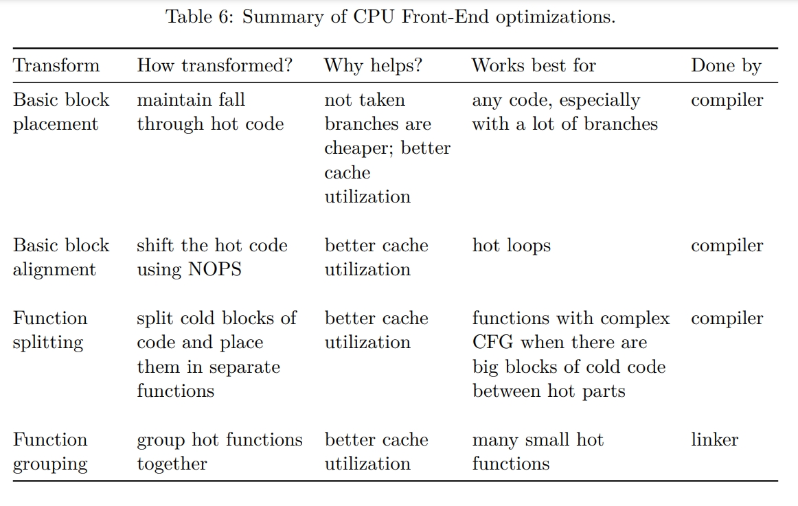
Basic block placement
1 | // hot path |
原因:
- Not taken branches are fundamentally cheaper than taken.
In the general case, modern Intel CPUs can execute two untaken branches per cycle but only one taken branch every two cycles. - 右边这幅图能够更好地利用 instruction cache 和 uop cache(之前提到的 DSB)。这是因为如果把所有的 hot code 连起来,就没有 cache line fragmentation。L1I Cache 中的所有的 Cache line 都被 hot code 使用。这点对 uop cache 也是一样的,因为它的 cache 也是基于下层的 code layout。
- 如果 taken branch 了,CPU 的 fetch 部分也会受影响。因为它也是 fetch 连续的 16 bytes 指令的。
通过指定 likely 和 unlikely 可以帮助编译器优化。如果一个分支是 unlikely 的,编译器可能选择不 inline,从而减少大小。likely 还可以在 switch 中使用。
Basic block alignment
Skylake 的 instruction cache line 的大小是 64 bytes,下面的代码可能被编译得跨越两个 cache line。这对 CPU 前端的性能会有影响,特别是像这种小循环。
1 | void benchmark_func(int* a) { |
下面的优化通过添加 nop 指令让整个循环都在一个缓存行里面。为什么这能提高性能比较复杂,因此就不解释了。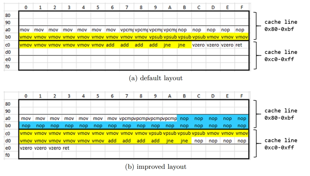
By default, the LLVM compiler recognizes loops and aligns them at 16B boundaries,就和上面图中未优化的情况一样。通过指定 -mllvm -align-all-blocks 可以变成优化后的样子。但是要慎重做这样的处理,因为增加 NOP 指令会影响执行时间。尽管 NOP 不执行,但是他同样需要被 fetch、解码、retire。所以需要额外地耗费在 FE 中的空间。
Function splitting
目的是将 hot 部分和 cold 部分分离出来。
1 | void foo(bool cond1, bool cond2) { |
分离后
1 | void foo(bool cond1, bool cond2) { |
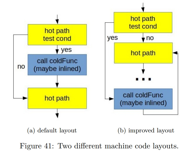
如下图所示,因为在 hot path 中只保留了 CALL,所以下一条指令很有可能在同一个 cache line 里面。这也说明了,对冷代码而言,应该避免它被 inline。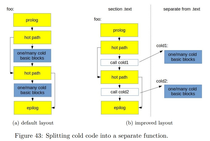
特别地,冷函数可以被放在 .text.old 中,从而避免在运行时加载。
Function grouping
Figure 44 gives a graphical representation of grouping foo, bar, and zoo. The default layout (see fig. 44a) requires four cache line reads, while in the improved version (see fig. 44b), code of foo, bar and zoo fits in only three cache lines. Additionally, when we call zoo from foo, the beginning of zoo is already in the I-cache since we fetched that cache line already.

和之前一样,function grouping 能提高 I-Cache 和 DSB-cache 的效率。
使用 ld.gold 链接器来指定顺序:
-ffunction-sectionsflag, which will put each function into a separate section.--section-ordering-file=order.txtoption should be used to provide a file with a sorted list of function names that reflects the desired final layout.
一个叫 HFSort 的工具可以帮助 group function。
Profile Guided Optimizations
Optimizing for ITLB
Virtual-to-physical address translation of memory address 也影响了 CPU FE 的效率。通常,这是被 TLB 来处理,TLB 会缓存最近的地址。When TLB cannot serve translation request, a time-consuming page walk of the kernel page table takes place to calculate the correct physical address for each referenced virtual address.
如果 TMA 指示了 high ITLB overhead,那么下面的内容就很重要:
- 将一些 performance-critical code 中的部分映射到较大的 page 中。
- 使用一些标准的 I-cache performance 优化办法,例如 reorder 函数让 hot 函数更为 collocated。或者通过 LTO 或者 IPO 技术减少 hot region 的大小。或者使用 profile guided optimization。或者使用激进的 inline 技术。
总结
CPU Back-End Optimizations
Most of the time, inefficiencies in CPU BE can be described as a situation when FE has fetched and decoded instructions, but BE is overloaded and can’t handle new instructions. Technically speaking, it is a situation when FE cannot deliver uops due to a lack of required resources for accepting new uops in the Backend. An example of it may be a stall due to data-cache miss or a stall due to the divider unit being overloaded.
I want to emphasize to the reader that it’s recommended to start looking into optimizing code for CPU BE only when TMA points to a high “Back-End Bound” metric. TMA further divides the Backend Bound metric into two main categories: Memory Bound and Core Bound, which we will discuss next.
Memory Bound
如下图所示,截止 2010 年,CPU 的提升比内存的提升要快很多。【Q】最近还是这样么?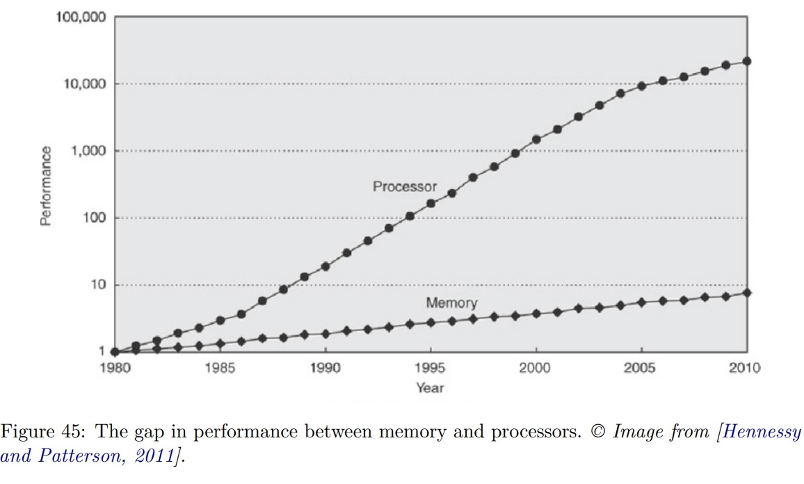
通过 TMA,Memory Bound estimates a fraction of slots where the CPU pipeline is likely stalled due to demand load or store instructions。
Cache-Friendly Data Structures
A variable can be fetched from the cache in just a few clock cycles, but it can take more than a hundred clock cycles to fetch the variable from RAM memory if it is not in the cache.
下面一张图展示了各个 CPU 操作的耗时。
Cache-friendly code 的关键是 temporal 和 spatial locality。
Access data sequentially
让 HW Prefetcher 感知到我们在顺序访问,从而提前取出下一个 chunk 的数据。
下面代码之所以是 cache friendly 的,是因为它的访问模式和它存储的 layout 是一致的。
1 | for (row = 0; row < NUMROWS; row++) |
又比如,传统的二分查找算法并没有很好的空间局部性,因为它会测试彼此之间相距很远的元素,这些元素可能在不同的 cache line 上。一个解决方案是使用 Eytzinger layout。我理解就是存在一个类似二叉堆的结构中。
Use appropriate containers
或者说是在 array 中直接存对象,还是存指针。如果排序,适合存指针。如果仅仅是线性遍历,适合存对象。
Packing the data
- 位域
- 重新排列 field 以减少 padding 和 aligning 带来的内存浪费
1
2
3
4
5
6
7
8
9
10struct S1 {
bool b;
int i;
short s;
}; // S1 is sizeof(int) * 3
struct S2 {
int i;
short s;
bool b;
}; // S2 is sizeof(int) * 2
Aligning and padding
比如,一个 16 bytes 的对象可能占用两个 cache line。读取这样的对象需要读两次 cache line。
A variable is accessed most efficiently if it is stored at a memory address, which is divisible by the size of the variable.
1 | // Make an aligned array |
Padding 技术还可以备用来解决 cache contention 和 false sharing 问题。
For example, false sharing issues might occur in multithreaded applications when two threads, A and B, access different fields of the same structure. An example of code when such a situation might happen is shown on Listing 24. Because a and b members of struct S could potentially occupy the same cache line, cache coherency issues might significantly slow down the program.
1 | struct S { |
通过 padding 来解决伪共享
1 |
|
When it comes to dynamic allocations via malloc, it is guaranteed that the returned memory address satisfies the target platform’s minimum alignment requirements. Some applications might benefit from a stricter alignment. For example, dynamically allocating 16 bytes with a 64 bytes alignment instead of the default 16 bytes alignment. In order to leverage this, users of POSIX systems can use memalign API.
Dynamic memory allocation
- 使用诸如 jemalloc 或者 tcmalloc 的实现
- 使用 custom allocator
例如 arena allocator。这样 allocator 不需要在每次分配的时候都 sys call。
另外,也更灵活,支持不同的策略。比如冷数据一个 arena,热数据一个 arena。将热数据放一起可以有机会共享 cache line。从而提高内存贷款和 spatial locality。同时还可以提高 TLB 利用率,因为 hot data 会占用更少的 page。
此外,还是 thread-aware 的,可以实现 thread local 的分配策略,从而避免线程间的同步。
Tune the code for memory hierarchy
这里还是 loop blocking 的例子。也就是将 matrix 切成多个小块,让每一块能够被装在 L2 cache 里面。
Explicit Memory Prefetching
如下代码所示,如果 calcNextIndex 返回的是很随机的数字,那么 arr[j] 会频繁 cache miss。如果 arr 很大,那么 HW prefetcher 就不能去识别 pattern,然后 prefetch。
因为在计算 j 和访问 arr[j] 之间有不少操作,所以可以借助 __builtin_prefetch 来 prefetch。这也是要点,一定要提前足够的时间。但也不能提前太多,从而污染 cache。在后面的 6.2.5 节中会介绍如何选择。
1 | for (int i = 0; i < N; ++i) { |
一般比较通用的是提前获取下一个 iter 的数据
1 | for (int i = 0; i < N; ++i) { |
需要注意,Explicit Memory Prefetching 不是 portable 的。可能在别的平台上反而会让性能变差。Consider a situation when we want to insert a prefetch instruction into the piece of code that has average IPC=2, and every DRAM access takes 100 cycles. To have the best effect, we would need to insert prefetching instruction 200 instructions before the load. It is not always possible, especially if the load address is computed right before the load itself. The pointer chasing problem can be a good example when explicit prefetching is helpless.
另外,prefetch 指令会加重 CPU 前端的开销。
Optimizing For DTLB
如前介绍,TLB is a fast but finite per-core cache for virtual-to-physical address translations of memory addresses. 没有它,每次内存访问都需要去遍历内核的 page table,然后计算出正确的 physical address。
TLB 由 L1 ITLB(instructions)、L1 DTLB(data) 和 L2 STLB(shared by data and instructions) 组成。L1 ITLB 的 cache miss 的惩罚很小,通常能够被 OOO 执行掩盖掉。L2 STLB 的 cache miss 就会导致遍历内核的 page table 了。这个 penalty 是可被观测的,因为这段时间 CPU 是 stall 的。假设 Linux 的默认 page size 是 4KB,L1 TLB 只能够存几百个 entry,覆盖大约 1MB 的地址空间。L2 STLB 覆盖大概一千多个。
一种减少 ITLB cache miss 的方案是使用更大的 page size。TLB 也支持使用 2MB 和 1GB 的 page。
Large memory applications such as relational database systems (e.g., MySQL, PostgreSQL, Oracle, etc.) and Java applications configured with large heap regions frequently benefit from using large pages.
On Linux OS, there are two ways of using large pages in an application: Explicit and Transparent Huge Pages.
Explicit Hugepages
用户可以通过 mmap 等指令去访问。可以通过 cat /proc/meminfo 并检查 HugePages_Total 来检查相关配置。
Huge page 可以在系统启动,或者运行的时候被保留。在启动期间保留的成功率更高,因为此时系统的内存空间没有被显著碎片化(fragmented)。
可以通过 libhugetlbfs 来 override 掉 malloc 调用。只需要调整环境变量酒席了。
- mmap using the MAP_HUGETLB flag
https://elixir.bootlin.com/linux/latest/source/tools/testing/selftests/vm/map_hugetlb.c - mmap using a file from a mounted hugetlbfs filesystem
https://elixir.bootlin.com/linux/latest/source/tools/testing/selftests/vm/hugepage-mmap.c - shmget using the SHM_HUGETLB flag
https://elixir.bootlin.com/linux/latest/source/tools/testing/selftests/vm/hugepage-shm.c
Transparent Hugepages
Linux also offers Transparent Hugepage Support(THP)。
1 | $ cat /sys/kernel/mm/transparent_hugepage/enabled |
always 表示 system wide,madvise 表示 per process。
Explicit vs. Transparent Hugepages
- Background maintenance of transparent huge pages incurs non-deterministic latency overhead from the kernel as it manages the inevitable fragmentation and swapping issues. EHP is not subject to memory fragmentation and cannot be swapped to the disk.
- EHP is available for use on all segments of an application, including text segments (i.e., benefits both DTLB and ITLB), while THP is only available for dynamically allocated memory regions.
Core Bound
也就是在 OOO 执行过程中所有不是因为内存原因造成的 stall。包含:
- Shortage in hardware compute resources
比如除法和平方根计算被 Divider Unit 处理,耗时比较长。如果这方面的操作比较多,那么就会造成 stall。 - Dependencies between software’s instructions
Inlining Functions
它不仅能够去掉调用函数的开销,同时也让其他优化变为可能。因为此时编译期能看到更多的代码。
对 LLVM 编译期而言,基于 computing cost 和 a threshold for each function call(callsite) 来计算。如果 cost 比 threshold 更低,就会 inline。
threshold 的选取通常是固定的,一般来说有一些启发式的方法:
- 小函数基本总是会被 inline
- 只有一个 callsite 的函数会被倾向于 inline
- 大函数通常不会 inline,因为它们让 caller 变大
有些不能 inline 的情况:
- 递归函数不能 inline
- Function that is referred to through a pointer can be inlined in place of a direct call but has to stay in the binary, i.e., cannot be fully inlined and eliminated. The same is true for functions with external linkage.
One way to find potential candidates for inlining in a program is by looking at the profiling data, and in particular, how hot is the prologue and the epilogue of the function. 下面的 demo 中,这个函数的 profile 中体现了 prologue 和 epilogue 花费了大概 50% 的时间。这可能说明了如果我们 inline 这个函数,就能减少 prologue 和 epilogue 的开销。但这不是绝对的,因为 inline 会导致一系列变化,所以很难预测结果。
1 | Overhead | Source code & Disassembly |
Loop Optimizations
通常,循环的性能被下面几点限制:
- memory lantency
- memory bandwidth
- 机器的 compute capability
Roofline Perfoemance Model 是评估 HW 理论最大值和不同的 loop 实际之间的方法。Top-Down Microarchitecture Analusis 是另外一个瓶颈相关的信息来源。
这一节中,首先讨论 low-level 的优化,也就是将代码在一个 loop 中移动。这样的优化方式让循环内的计算更有效率。然后是 high-level 的优化,会 restructure loops,通常会影响多个 loop。第二种优化的目的主要是提高 memory access。eliminating memory bandwidth 和 memory lantency 问题。
Low-level optimizations
下面这些优化通常能够提高具有 high arithmetic intensity 的 loop 的性能,比如循环是 CPU-compute-bound 的。大部分情况下,编译器能够自己做相关优化,少部分情况下,需要人工帮助。
Loop Invariant Code Motion (LICM)
将循环中的不变量移出循环。
什么是循环中的不变量呢? Expressions evaluated in a loop that never change are called loop invariants.
1 | for (int i = 0; i < N; ++i) |
Loop Unrolling
循环的 induction variable,也就是 for i 的那个 i,每个 iteration 去修改它的代价是比较大的。所以可以选择 unroll 一个循环。
下面的例子中,unroll the loop by a factor of 2. 从而减少了 compare 和 branch 指令的开销到原来的一半。
1 | for (int i = 0; i < N; ++i) |
作者建议不要手工展开循环:
- 编译器很擅长做这个,并且做得很好
- 处理器有一个 “embedded unroller”,thanks to their OOO speculative execution engine
当处理器正等待第一个 iteration 的负载完成时,它可能预先开始执行第二个 iteration 的负载了。This spans to multiple iterations ahead, effectively unrolling the loop in the instruction Reorder Buffer (ROB).
Loop Strength Reduction (LSR)
将开销比较大的操作换为开销更小的操作。通常和 induction variable 上的计算有关。
1 | for (int i = 0; i < N; ++i) |
Loop Unswitching
这个很简单,尝试能不能把 loop 中的 branch 提出来,分成两个 loop
1 | for (i = 0; i < N; i++) { |
High-level optimizations
下面的一些变换,从编译器的角度比较难合法地或者自动地进行。所以很多时候可能需要手动做。
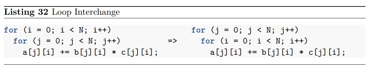
Loop Interchange
交换多层循环的 order。
目的是 perform sequential memory accesses to the elements of a multi-dimensional array。
如下所示,在一个按行存储的数组中,让 i 到内层循环的空间局部性更好。
Loop Blocking (Tiling)
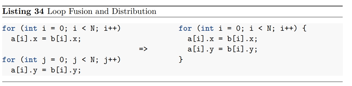
Loop Fusion and Distribution (Fission)
Loop fusion 可以用来:
- 减少 loop overhead,因为它会复用相同的 induction variable
- 可以提高 memory access 的 temporal locality
如下代码中,如果 x 和 y 都位于同一个缓存行上面,那么将两个 loop fuse 在一起能够避免加载同一个缓存行两次。
这样就能减少 cache footprint,并且提高 memory bandwidth utilization。
相反地有 Loop Distribution 即 Loop Fission。其目的是:
- 可以先在一个循环中 pre-filter、sort、reorg 数据
- 减少一个 iteration 中需要访问的数据,从而提高 memory access 的 temporal locality。这对具有较高 cache contention 的场景,也就是大 loop 中会比较有用
- 减少对寄存器的压力,同样是因为一个 iteration 中会执行更少的操作了
- 通常还可能提升 CPU FE 的性能,因为 cache utilization 会更好
- 编译期能够更好地优化小循环
Discovering loop optimization opportunities
如下所示,编译器不能把 strlen 移出循环体。这是因为 a 和 b 两个数组可能是 overlap 的。所以,需要通过 restrict 关键词来显式声明这两段内存不会 overlap。
1 | void foo(char* a, char* b) { |
在一些时候,编译期可以通过 compiler optimization remarks (sec 5.7) 告诉我们失败了的优化。但对于上面的情况,Clang 10 和 GCC 10 目前还都不行。目前只能通过反编译出来的代码才能看出来。
有一些指令可以配置编译器的优化行为,例如 #pragma unroll(8)。
Use Loop Optimization Frameworks
目前有一些框架可以检测 loop transformation 的合法性了。例如 polyhedral 框架,polyhedral 的意思是多面体。LLVM 系列也有自己的 polyheral 框架,即 Polly。LLVM 默认不启用。对于 GEMM 内核,Polly 能提供 20 倍左右的提速。
Vectorization
大部分情况下,Vectorization 能够被编译器发现,然后自动发生。
一般来说,在编译器中完成三种 Vectorization:
- inner loop vectorization
- outer loop vectorization
- SLP (Superword-Level Parallelism) vectorization
第一种最常见。
Compiler Autovectorization
阻止 Autovectorization 的情况:
- unsigned loop-indices 溢出
- 两个指针可能指向重叠的内存区间
- 处理器本身不支持比如 predicated (bitmask-controlled) load and store operation
- vector-wide format conversion between signed integers to doubles because the result operates on vector registers of different sizes
所以一般分为三步:
- Legality-check
检查 the loop progresses linearly。
确保 the memory and arithmetic operations in the loop can be widened into consecutive operations。
That the control flow of the loop is uniform across all lanes and that the memory access patterns are uniform。没看懂是在说什么。
确保不会访问和修改不应该的内存。
analyze the possible range of pointers, and if it has some missing information, it has to assume that the transformation is illegal。看不懂。 - Profitability-check
It needs to take into account the added instructions that shuffle data into registers, predict register pressure, and estimate the cost of the loop guards that ensure that preconditions that allow vectorizations are met. 我觉得作者这样说就是在让人看不懂。 - Transformation
Discovering vectorization opportunities
检查 compiler vectorization remarks 可以发现编译期进行了什么优化,包含是否 vectorized 了,vectorization factor(VF) 是多少。
Vectorization is illegal
下面的函数不是 vectorizable 的。因为是 read-after-write dependence.
1 | void vectorDependence(int *A, int n) { |
下面的函数不是 vectorizable 的。因为是 floating-point arithmetic。一般来说,浮点数加法是可交换的,但浮点数加法不是可结合的。如果向量化,则会导致不同的 round decision,和一个不同的结果。
1 | float calcSum(float* a, unsigned N) { |
如下所示的代码,GCC 会为其创建两个不同的版本。如果发现 a 和 b 和 c 有 overlap,则运行普通版本,否则运行 simd 版本。
1 | void foo(float* a, float* b, float* c, unsigned N) { |
输出
1 | $ gcc -O3 -march=core-avx2 -fopt-info |
Vectorization is not beneficial
1 | void stridedLoads(int *A, int *B, int n) { |
Loop vectorized but scalar version used
一般是因为 loop trip 比较小。比如以 AVX2 来说,如果同时加上 unroll 循环的技术,假设 unroll 4-5 倍,那么一个 loop iteration 需要处理 40 个元素。所以这种情况下,会直接 fallback 到处理剩余尾数的普通循环中。
此时,可以强制使用更小的 vectorization factor 或者 unroll count。
1 |
Loop vectorized in a suboptimal way
最优的 vectorization factor 是难以通过直觉判断的,因为存在以下因素:
- 很难在大脑中模拟 CPU 的运行模式
Vector shuffles that touch multiple vector lanes could be more or less expensive than expected, depending on many factors.
什么是 vector shuffle? - 运行时,程序可能以非预期的方式运行,取决于 port pressure 或者其他因素
人类可以通过 Vectorization pragmas 来尝试各种 vectorization factor。也可以尝试各种 unroll factor 来选出最优的。但编译器做不到。 - 非 vec 的版本可能更好
因为 gather/scatter loads, masking, shuffle 这些向量操作更昂贵。
所以也需要尝试禁用向量化比较性能。如使用-fno-vectorize和-fno-slp-vectorize,或者#pragma clang loop vectorize(enable)。
Use languages with explicit vectorization
“Close to the metal” programming model
这里说的是传统的 C 和 C++ 中没有向量化的概念,所以总是需要通过 compiler intrinsics 来做这个工作。而像 ISPC 这样的语言中 += 这样的操作符会被隐式地认为是 SIMD 操作,并会并行的执行多个加法。
Optimizing Bad Speculation
Mispredicting a branch can add a significant speed penalty when it happens regularly. When such an event happens, a CPU is required to clear all the speculative work that was done ahead of time and later was proven to be wrong. It also needs to flush the whole pipeline and start filling it with instructions from the correct path. Typically, modern CPUs experience a 15-20 cycles penalty as a result of a branch misprediction.
现在的处理器能够进行分支预测,不仅仅是静态的规则,甚至可以发现动态的模式。
我们可以通过 TMA Bad Speculation 指标来查看一个程序在多大程度上收到分支预测的影响。对此,作者推荐只有当分支预测失败率在 10% 以上的时候,再进行关注。
从前,可以在分治命令前加上前缀 0x2E 或者 0x3E 来分别表示是否选择这个分支。但随着后面分支预测机制的完善,这个功能被去掉了。所以目前唯一能够避免分支预测失败的直接办法是不使用分支。下面介绍两种避免分支的办法。
注:likely 和 unlikely 是通过放置可能性较大的指令到靠近分支跳转指令来实现优化的。
Replace branches with lookup
1 | int mapToBucket(unsigned v) { |
Replace branches with predication
额外说明
superscalar 和 SMT
在“Superscalar Engines and VLIW”中介绍了 superscalar 技术。superscalar 指的是在一条流水线中,有多个执行单元,所以在一个 cycle 中可以 issue 多条指令。所以这就导致原先串行的命令中,不冲突的命令不再构成全序关系,这也就是所谓的 OOO 乱序执行。BTW,将全序关系拆解成多个不冲突的偏序关系也是一种并行或者分布式领域的常用技术。
SMT 也就是 Simultaneous Multithreading,也被称为 hyperthreading。指一个核心同时拥有两套寄存器、缓存,保存两个线程工作的现场。