本部分开始为最新的学习笔记。包含 PolarDB Serverless、Monkey: Optimal Navigable Key-Value Store、Are You Sure You Want to Use MMAP in Your Database Management System、SLM-DB: Single-Level Key-Value Store with Persistent Memory
PolarDB Serverless: A Cloud Native Database for Disaggregated Data Centers
https://users.cs.utah.edu/~lifeifei/papers/polardbserverless-sigmod21.pdf
INTRODUCTION
大概有三种 cloud 数据库的架构:
- monolithic
- virtual machine with remote disk
- shared storage
后两种也被统称为存算分离的架构。
存算一体的架构缺点:
- 将 db 分配到对应的机器类似于解决 bin-packing 问题
- 难以满足客户的灵活的资源需要
- 资源之间没法独立地进行恢复
下面两种存算分离的架构:CPU 和内存同样存在 bin-packing 的问题,内存开销大。
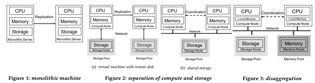
因此 PolarDB Serverless 共享了内存。
和 Aurora、HyperScale 以及 PolarDB 一样,它有一个 RW 的主节点,以及多个 read only replica。它也可以通过提出的 disaggregation 架构支持多个 RW 主节点,但不在这个论文中讨论。
一些挑战:
- 引入共享内存后,事务的正确性。
- read after write 不会在节点间丢失修改 -> cache invalidation
- RW 节点在 split 或者 merge 一个 B+Tree 的时候,其他的 RO 节点不能看到一个不一致的 B 树 -> global page latch
- 不能脏读 -> 在不同的 database node 间同步 read view
- 网络延迟
- 使用 RDMA CAS 技术提优化 global latch 的获取
- page materialization offloading 技术将 dirty page 从 remote memory 中驱逐,而不是将它们 flush 到存储中
BACKGROUND
PolarDB
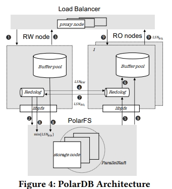
介绍了 PolarFS。
RW 和 RO 节点通过 redo log 同步内存状态。通过 LSN 实现一致性,其执行流程是:
- 将所有的 redo log flush 到 PolarFS 中
- 提交事务
- RW 异步广播消息:read log 以及最新的 LSN 即 LSN_rw。
- 当 ROi 收到 RW 的消息后,从 PolarFS 上拉取所有的 redo log,将它们 apply 到 buffer pool 中的 buffered page 里面
- ROi 此时就和 RW 完成了已同步
- ROi 将自己的 LSN_ro 发送给 RW
- RW 可以在后台将 read log 去 truncate 到所有的 LSN_roi 的最小值
- ROi可以处理 LSN_roi 之前的读取,提供 SI 隔离级别
假设某个 ROk 落后了,比方说落后超过 1M,这样的节点会被发现,并且被踢出集群。
Disaggregated Data Centers
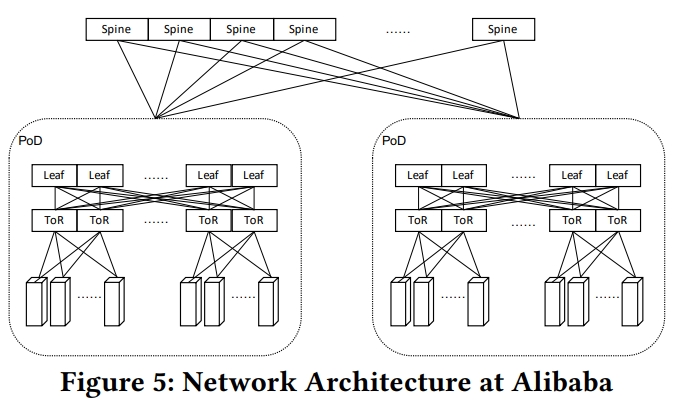
在 disaggregation 架构下,一个数据库实例所需要的计算、内存和存储资源将被分配到同一个 PoD 下面。不同的 db instance 则看见恶意分配到不同的 PoD 下面。计算和内存资源会被尽可能分配到同一个 ToR 下面。
一台机器有两个 RDMA NIC,他们会被连接到两个 ToR 交换机上面,从而避免网络连接失效。一个 leaf switch group 由多个 leaf switch 组成。ToR switch 连接到 leaf switch 上。
Serverless Databases
pay-as-you-go model。
一个 ACU 包含了 2GiB 的内存以及对应的虚拟处理器。这个设定 fixes the resource ratio。比如,分析数据库可能需要更多的内存,而不是 CPU,因为它们可能要 cache 大量的数据。对应的,事务数据库需要大量的 CPU 去处理业务的尖峰。而一个小内存,只要能满足 cache hit,那也是足够的了。
DESIGN
Disaggregated Memory
Remote Memory Access Interface
这里内存也是按照 Page 来组织的。一个 PageID 可以表示为 (space, page_no)。使用 page_register 和 page_unregister 去做类似 RC 一样的内存管理。page_read 从 remote memory pool 拉数据到 local cache。page_write 将 page 从 local cache 写到 remote memory pool。page_invalidate 被 RW 调用,用来将所有 RO 的 local cache 上的 page 设置为无效。
Remote Memory Management
内存分配的单位是 slab,一个 slab 是 1Gb。
Page Array(PA)
一个 slab 被一个 PA 结构实现。一个 PA 是一个连续的内存,包含 16KB page 的 array。PA 中的 page 可以被 remote node 通过 RDMA 直接访问,因为他们在启动的时候就已经被注册到 RDMA NIC 上了。
一个 memory node 也被称为一个 slab node。一个 slab node 管理多个 slab。一个实例可以对应到多个 slab node 上,其中第一个 slab node 称为 home node。home node 中有一些 instance 级别的元数据。
Page Address Table (PAT)
PAT is a hash table that records the location (slab node id and physical memory address) and reference count of each page. 也就是前面 page_register 和 page_unregister 所操作的东西。
【Q】这个结构保存在哪里?
Page Invalidation Bitmap (PIB)
PIB is a bitmap. For each entry in the PAT table, there is an invalidation bit in PIB. Value 0 indicates that the copy of the page in the memory pool is of the latest version, while value 1 means that the RW node has updated the page in its local cache and haven’t written it back to the remote memory pool yet. There is also a local PIB on each RO node, indicating whether each page in the RO node’s local cache is outdated.
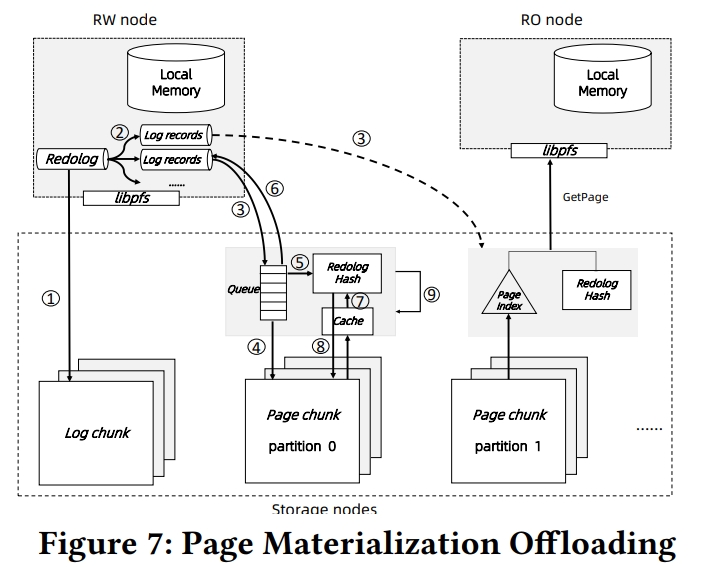
Page Materialization Offloading
Aurora 提出 log is database 的理论。将 redo log 看做是增量的 page 修改。Socrates 进一步地,将 log 从 storage 分离。Log 被存在 XLOG 服务中,然后被异步地发送到一系列 page server 中,每一个 page server 负责一个 database partition,独立地重放日志,生成 page 并处理 GetPage@LSN 请求。
PolarDB 类似于 Socrates,将 PolarFS 设计为分别存放 log 和 page 到两个 chunck 中。redo log 首先被持久化到 log chunkc 中,然后被异步地发送到 page chunck 中。在 page chunck 中,logs 被 apply,从而更新 page。不同于 Socrates,为了重用 PolarFS,log 只会被发送到 page chunk 的 leader 节点,这个节点会物化 page,然后将 update 通过 ParallelRaft 通知给其他的 replica。This method adds additional latency to the ApplyLog operation due to the replication cost. However, it is not a critical issue because ApplyLog is an asynchronous operation not in the critical path. Moreover, since the replicated state machine guarantees data consistency between page chunks, there is no need for an extra gossip protocol among storage nodes like in Aurora.
Monkey: Optimal Navigable Key-Value Store
https://nivdayan.github.io/monkeykeyvaluestore.pdf
个人觉得一篇很好的文章,介绍了 LSM 的 design space。
Abstract
Bloom filter 的 FP 率,和最坏情况下的查询开销成正比。
The insight is that worst-case lookup cost is proportional to the sum of the false positive rates of the Bloom filters across all levels of the LSM-tree.
对于不同的层,引入不同的 bloomfilter 的大小。
Monkey allocates memory to filters across different levels so as to minimize this sum.
设计了一个调优工具。感觉类似 《Fast Scans on Key-Value Stores》里面的思路。
Furthermore, we map the LSM-tree design space onto a closed-form model that enables co-tuning the merge policy, the buffer size and the filters’ false positive rates to trade among lookup cost, update cost and/or main memory, depending on the workload (proportion oflookups and updates), the dataset (number and size of entries), and the underlying hardware (main memory available, disk vs. flash). We show how to use this model to answer what-if design questions about how changes in environmental parameters impact performance and how to adapt the various LSM-tree design elements accordingly.
INTRODUCTION
The intuition is that any given amount of main memory allocated to Bloom filters of larger runs brings only a relatively minor benefit in terms of how much it can decrease their false positive rates (to save I/Os). On the contrary, the same amount of memory can have a higher impact in reducing the false positive rate for smaller runs.
调研 Pareto curve 基于内存容量和工作负载,去寻找到查询和更新开销的平衡点。
The second key point in Monkey is navigating the Pareto curve to find the optimal balance between lookup cost and update cost under a given main memory budget and application workload (lookup over update ratio).
BACKGROUND
Buffering Updates
首先是下面这张图。
$M_{buffer}$ 等于 $ P \times B \ times E$。E 是 entry 的大小,B 是一个 disk page 中有多少个 entry,P 是内存中有多少个 disk page 用于 buffer。
$ N \times \frac{T-1}{T} $ 是怎么来的呢?其实是个等比数列求和
1 | 1 + T + T^2 + ... + T^(L-1) + T^L = N |
套一下公式,然后取 T^L-1 直接约等于 T^L,即可得到结果。
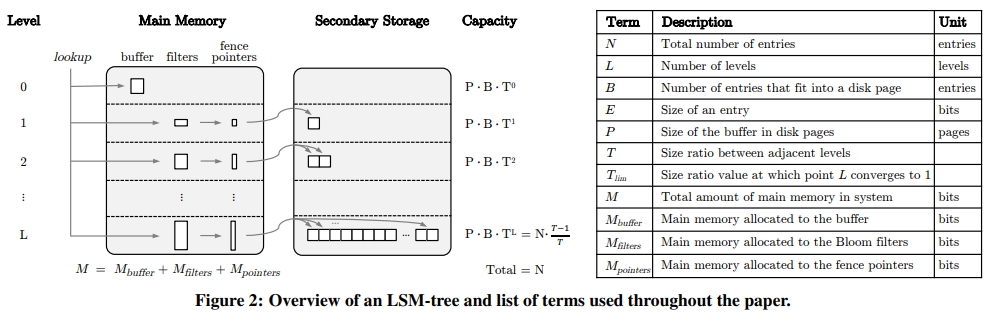
然后,得到另一个 L 关于 T 的公式。
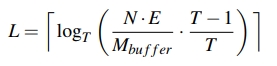
其中,T 是有一个上限的取值,即 $ \frac{N \times E}{M_{buffer}} $。取这个上限时,L 会退化到 1。因为整个数据库才 $ N \times E $ 这么大,挨个按照 tiered 逻辑 dump 下来就是公式这么多个,然后 T 等于它,那么这一层永远将将好填满。
Merge Operations
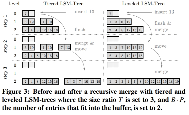
The essential difference is that a leveled LSM-tree merges runs more greedily and therefore gives a tighter bound on the overall number of runs that a lookup has to probe, but this comes at the expense of a higher amortized update cost.
Lookups
查询从 buffer 开始,从低层往高层走。一旦找到第一个满足要求的就可以立即返回,因为层数越往下,数据是越旧的。
A point lookup starts from the buffer and traverses the levels from lowest to highest (and the runs within those levels from youngest to oldest in the case of tiering). When it finds the first matching entry it terminates. There is no need to look further because entries with the same key at older runs are superseded.
- 查找一个不存在的值代价可能很高,因为会检查所有 level 中的所有 run
- 范围查询需要 sort merge 一系列 run,然后丢掉被 override 掉的数据
Probing a Run
在 1996 年最老的 LSM 设计中,每个 run 是被存储为压缩的 B 树的。
Over the past two decades, however, main memory has become cheaper, so modern designs simply store an array of fence pointers in main memory with min/max information for every disk page of every run.
Maintaining a flat array structure is much simpler and leads to good search performance in memory (binary search as each run is sorted).
查询的时候,
- 如果是点查,那么就先二分 fencing pointers,然后找到对应的 page
- 如果是扫表,也还是二分到对应的 page,然后从这个 page 往后读取
所以,如果只需要 O(1) 的 disk IO,那么 pointers 的内存大概是 O(N / B)。
For example, with 16 KB disk pages and 4 byte pointers, the fence pointers are smaller by ≈ 4 orders of magnitude than the raw data size. Stated formally, we denote the amount of main memory occupied by the fence pointers as $M_{pointers}$, and we assume throughout this work that $M_{pointers}$ is
O(N / B)thereby guaranteeing that probing a run takesO(1)disk I/O for point lookups.
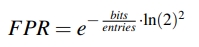
Bloom Filters
FPR 即假阳性率,和 entry 的数量正相关,和 bloom filter 的内存占用负相关。如下面公式所示,其中 entries 表示一个 run 中的 entry 的数量,bits 表示内存中用作这个 run 的 Bloomfilter 的大小。
具体算法可以看我的文章。
因为如果出现假阳性,则需要去下一个 sst 文件(tiered)或者下一层(leveled)中去找下一个 run。因此假阳性率实际上就关系到找一个 key 要有多少次 disk IO,从而直接影响到性能。
Rocksdb 中普遍使用 10 bits 给 Bloomfilter,则假阳性率在 1%。
Cost Analysis
如何度量最坏情况呢?
- 对于 update,度量 amortized worst-case I/O cost,主要和 update 之后的 merge 操作有关
- 对于 lookup,度量 zero-result average worst-case I/O cost。原因是它很常见,并且它的 IO overhead 确实很大
对于最坏情况:
- Tierd
- Lookup 的 IO 正比于 L、T、FPR 三者乘积
- Update 的 IO 正比于 L / B
- Leveled
- Lookup 的 IO 正比于 L、FPR 二者乘积
- Update 的 IO 正比于 T * L / B
下面这张表中,从 Log 到 Sorted Array,数据越来越有序,但付出的整理的代价也越来越大。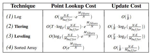
它的计算过程在下面这段话中,其中 $O(e^{-\frac{M_{buffers}}{N}})$ 就是上面的 FPR。其中 $M_{buffers}$ 和 bits 成正比,$N$ 和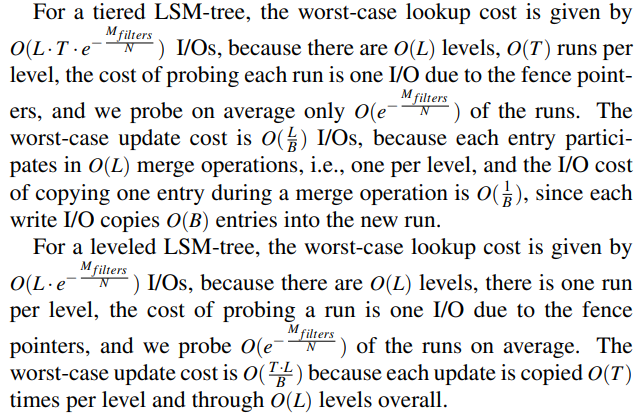
LSM-TREE DESIGN SPACE
The design space of LSM trees spans everything between a write-optimized log to a read-optimized sorted array.
Tuning the Merge Policy and Size Ratio
Figure 4 是一个很有趣的图。虚线部分是 Tiering 策略的 update 和 lookup 开销随着 T 变化的情况。可以看到,Tiering 策略总体是偏向于写优化的,它读写最优的点,即 T = 2 的时候,也将将才和 Leveling 策略打平。
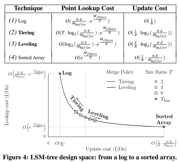
设置 T 为 2,那么 tiering 和 leveling 这两种策略的更新查找开销是相同的。
The first insight about the design space is that when the size ratio T is set to 2, the complexities of lookup and update costs for tiering and leveling become identical.
特别地,当 T 为 1,则总层数 L 为 1。也就是说这个 LSM 树会退化为 log。
We did not plot the curve to scale, and in reality the markers are much closer to the graph’s origin. However, the shape of the curve and its limits are accurate.
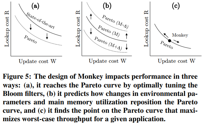
Tuning Main Memory Allocation
The limits of the curve in Figure 4 are determined by the allocation of main memory among the
filters $M_{filters}$ and the buffer $M_{buffer}$.
Design space contentions
- 如何将总共 $M_{filters}$ 这么多内存分配给所有的 Bloomfilter?
- 如何在 buffer 和 filter 之间分配内存?
例如,根据 Figure 4,如果分配在 buffer 上的内存变多,那么 lookup 和 update 的 cost 就会变低,但是会同时提高 Bloomfilter 的 FP 率,从而又实际上提高了 lookup 的 cost。 - 如何调节 size ratio 也就是 T 和 merge policy?
The State of the Art
All LSM-tree based key-value stores that we know of apply static and suboptimal decisions regarding the above contentions. The Bloom filters are all tuned the same, the Buffer size relative to the Bloom filters size is static, and the size ratio and merge policy are also static
MONKEY
综述
Design Knobs
Those knobs comprise:
- the size ratio among levels T
the merge policy (leveling vs. tiering) - the false positive rates p1…pL assigned to Bloom filters across different levels
- the allocation of main memory M between the buffer $M_{buffer}$ and the filters $M_{filters}$.
Minimizing Lookup Cost
主要是调整了各层的布隆过滤器的 FPR。
Performance Prediction
Auto tuning
- 在 4.3 中,用了渐进分析的办法
- 在 4.4 中,定义了最坏情况的吞吐,使用了
- 查找和更新开销
- 查找和更新的比例
- 在持久化存储中读取和写入的开销
Minimizing Lookup Cost
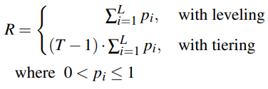
定义 R 是一个返回 0 结果集的点查的 IO 开销,也就是最坏的情况。
We first show that R is equal to the sum of the false positive rates (FPRs) of all Bloom filters.
We then show how to tune the Bloom filters’ FPRs across different levels to minimize this sum, subject to a constraint on the overall amount of main memory $M_{filters}$.
We assume a fixed entry size E throughout this section
in Appendix C we give a iterative optimization algorithm that quickly finds the optimal FPR assignment even when the entry size is variable or changes over time.
Modeling Average Worst-Case Lookup Cost
要扫描的 run 数,对应了所有 Bloomfilter 的 FPR 之和。如下所示,其中 pi 表示每一层的 FPR。
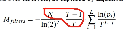
Modeling Main Memory Footprint
可以重写上面 FPR 的公式,得到 bits 和 FPR 的关系。
然后,从上面式子,可以根据每一层的 FPR 即 pi,推导出 $M_{filter}$ 的内存占用。
下面式子的红色框中,通过总的 entry 数量 N 推导出每一层 entry 的数量。因此,求和中的每一项,是每一层的 Bloomfilter 占用的内存。
Minimizing Lookup Cost with Monkey
Are You Sure You Want to Use MMAP in Your Database Management System?
mmap
https://man7.org/linux/man-pages/man2/mmap.2.html
INTRODUCTION
传统地,数据库使用一个 buffer pool 去维护从二级存储中读上来的数据。但是,现在有另一种使用 mmap 的选择:mmap 使得用户可以把数据库当成始终在内存中一样去使用。当内存不够时,旧的 page 可以被自动 evict 掉(这里应该指的是非 MAP_ANONYMOUS 的情况)。
看到这里,我个人觉得 mmap 有几点问题:
- 绑定了磁盘数据结构和内存数据结构。例如,磁盘中的数据可能会被压缩;内存数据结构更容易使用指针进行跳转。
- 无法控制落盘的时间。例如 这里记录的一个问题。
BACKGROUND
MMAP Overview
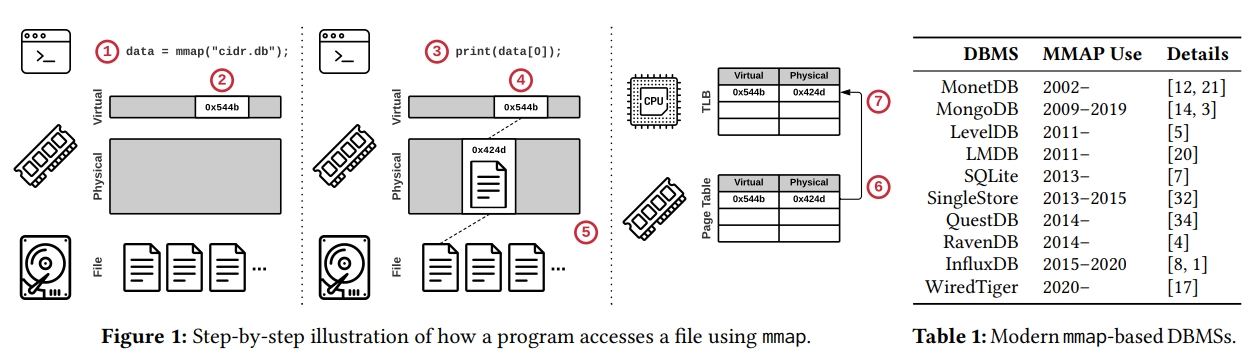
下图是一个基于 mmap 的数据库的通常的实现:
- 调用 mmap,得到一个指针
- 系统分配虚拟地址,但是不会真正的去读文件
- 程序通过指针去读文件
- 系统尝试去获取 page
- 因为目前还没有指向这个虚拟地址的 mapping,所以系统触发一个 page fault,去加载对应内存
- 系统在 page table 中添加了一个 entry,记录了虚拟地址到物理地址的映射
- Initialating CPU core 也会将这个 entry cache 在自己的 local translation lookaside buffer 即 TLB 中来实现加速访问
当 munmap 发生时,page 需要被 evict 掉,要做相反的事情:
- mapping 需要被 OS 移除
- CPU core 需要 flush TLB 中的 entry。对于 initiating core 这还是简单的,但同时还需要保证 remote core 中没有 stale entry。因为目前对于 remote TLB 没有 coherence,所以 OS 需要触发一个昂贵的 inter-processor 中断去 flush,这称为 TLB shootdown。
这里问了下 GPT 有关 TLB shootdown 的原理:
- 本地 TLB 刷新 :当一个虚拟到物理地址的映射在某个核的 TLB 中因为内存映射变化而变得过时时,操作系统会先将该过时的映射条目从本地 TLB 中刷新掉。
- 发送 IPI 中断 :接着,发起 TLB Shootdown 的核会向其他可能缓存有该过时映射的远程核心发送一种称为 IPI(Inter-Processor Interrupt,处理器间中断)的特殊中断信号。
- 远程 TLB 刷新并反馈 :远程核心接收到 IPI 中断后,会执行相应的中断处理程序来检查自己的 TLB,并将其中的过时条目进行无效化处理,完成后会向发起核发送一个完成反馈信号,以告知 TLB Shootdown 已经完成。
总而言之,就是页表发生变化的时候,就可能涉及 TLB Shotdown。
POSIX API
介绍一下相关的重要 API:
- mmap
MAP_SHARED 会导致共享。
MAP_PRIVATE 会导致 COW 机制。变更不会被写入到 backing file 中,也不会被其他 mmap 到同一个文件的进程看到。 - madvise
Hint 操作系统需要的访问模式。
MADV_NORMAL:OS 会取需要的页,以及 next 16 和 previous 15 个 page。如果一个 page 是 4KB,会导致 OS 读取 128KB,哪怕这个 caller 真的只需要用一个 page。
MADV_RANDOM:只会读需要的页。
MADV_SEQUENTIAL:从 mmap 的 man 文档中看到的说法是“aggressively read ahead”且“may be freed soon after they are accessed”。 - mlock
强制这个页面不能被 evict,一直在内存里面。
POSIX 标准和 Linux 的实现都允许 OS 在任何时候 flush dirty page 到 backing file 上。
因此,这个手段不能用来强制不刷脏页。 - msync
强制将 dirty page 刷到 backing file 上。
MMAP Gone Wrong
一些使用 mmap 的 DB:
- MonetDB 使用 mmap 存储独立的 column
- SQLite 提供一个选项,允许使用 mmap 而不是默认的 read write 系统调用
- LMDB 只使用 mmap
关于 MonetDB 的情况是,它在早期使用了 mmap,称为 MMAPv1 作为存储引擎。但是遇到一些问题:
- an overly complex copying scheme to ensure correctness
- the inability to perform any compression for data on secondary storage managed the file mapping, the in-memory data layout needed to match the physical representation on secondary storage, leading to wasted space and reduced I/O throughput
在 2015 年,MonetDB 使用 WiredTiger 替换了 MMAPv1。后续在 2020 年,WiredTiger 中重新引入了 mmap,但目的只是在特定的情况下减少跨内核和用户空间的开销。
InfluxDB is a time series DBMS that used mmap for file I/O in earlier releases [8]. However, the developers replaced mmap after observing I/O spikes for writes when a database grew larger than a few GB in size, likely due to the overheads associated with page eviction (Section 3.4). They also faced other issues when running in containerized environments or on machines without direct-attached storage (e.g., cloud deployments), which further precluded the use of mmap in their new IOx storage engine [1].
下面这个 SingleStore 的 case 不是很明白,mmap 的好处之一就是节省系统调用吧。mmap 只需要对需要读的文件调用一次即可,理论上不同的查询是可以 share 的。
SingleStore removed mmap-based file I/O after encountering poor performance on simple sequential scan queries [32]. The DBMS’s calls to mmap were taking 10–20 ms per query, which accounted for nearly half of the overall query runtime. Upon further investigation, the developers identified the source of the problem as contention on a shared mmap write lock. By switching to read system calls, the queries became fully CPU-bound.
LevelDB 的情况,可以看 NewRandomAccessFile 的实现,可以发现,尽管默认创建 PosixMmapReadableFile,但依然有个 mmap limiter 使得在一些场景下会回退到 PosixRandomAccessFile。
1 | // Currently used to limit read-only file descriptors and mmap file usage |
Facebook created RocksDB as a fork of Google’s LevelDB partly due to performance bottlenecks for reads caused by the latter’s use of mmap.
SLM-DB: Single-Level Key-Value Store with Persistent Memory
https://www.usenix.org/system/files/fast19-kaiyrakhmet.pdf
https://www.usenix.org/conference/fast19/presentation/kaiyrakhmet
Presentation
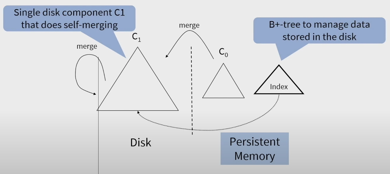
演讲里面的 Component 可以直接看成是 Level。
这个架构主要是:
- 因为使用了 persistent memory 作为 memtable,所以不需要 WAL 了
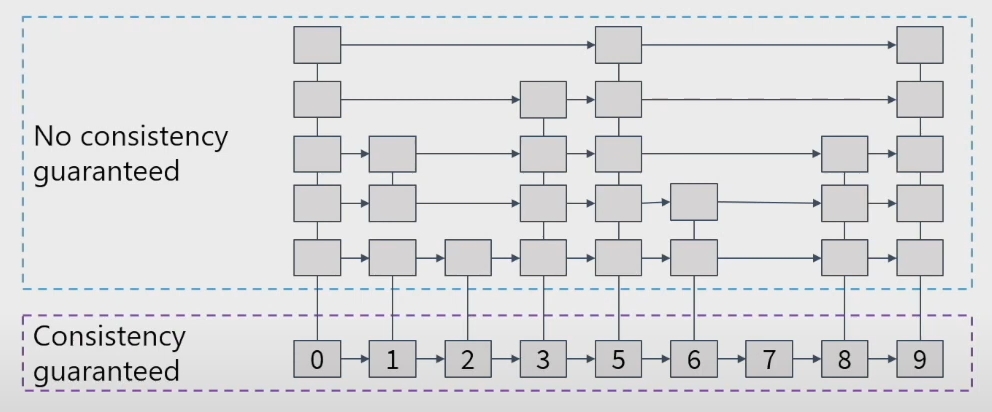
- 引入了一个 global 的 B+ 树索引。这样也不需要一个 multi level merge structure 了
- Selective Compaction 机制
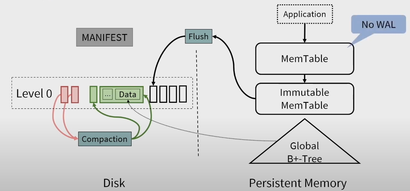
Memtable
当 Immutable 被 flush 到 disk 的时候,会写入 B+ 树的索引。
Compaction 的另一个目的是 Range Search 需要的顺序性。没怎么看明白

Live Key ratio selection 有点像 TiFlash 的 PS3 的实现。
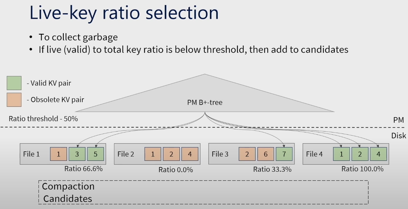
从论文里补充下计算方式:
- the total number of KV pairs stored in s is computed at creation, and initially the number of valid KV pairs is equal to the total number of KV pairs in s
- when we update a pointer to the new location object for the key in the B+-tree, we decrease the number of valid KV pairs in s
简单来说,如果 SST 里面的 kv pair 陈旧了,就说明它的新版本肯定被写到一个新的 SST 里面了。B+ 树能体现出这个变更。
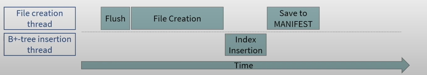
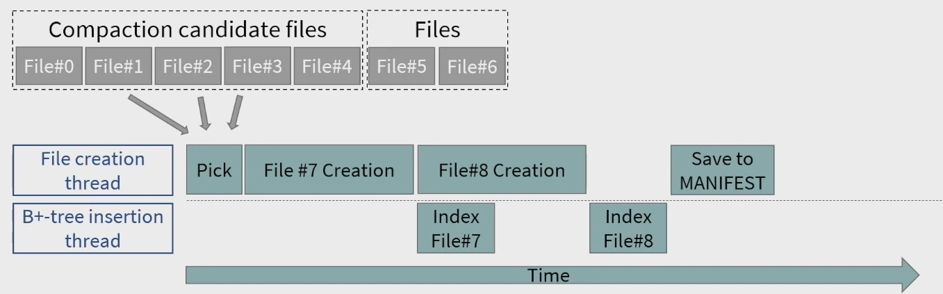
Compaction 的过程如下所示,主要是两个线程,一个线程 flush,一个线程构建 index。有点类似流水线一样。
个人理解
在内存中建立的 B+ tree 提高了 read 的效率,避免了之前一层一层往下找的开销。这样,就可以激进地将 LSM 减少到一层,减少 Compaction 的写放大。
Introduction
Single-Level Merge DB (SLM-DB)
Selective Compaction
compaction candidate list
overlapping ratio:对于 SST s,计算它和每个其他的 SST t 的 overlapping ratio。这是根据 s 和 t 各自的 head 和 tail 来算的,所以是比较快的,不需要遍历整个 SST。作者提出了一个公式,如果这个公式算出来是小于等于 0 的,那么就说明不 overlap。数据库会在后台异步地 compact s 和它 overlapping ratio 最大的 SST。
When merging multiple SSTable files, we need to check if each KV pair in the files is valid or obsolete, which is done
by searching the key in the B+-tree. If it is valid, we mergesort it with the other valid KV pairs. If the key does not exist in the B+-tree or the key is currently stored in some other SSTable, we drop that obsolete KV pair from merging to a new file.
leaf node 的这个优化指的应该是合并小文件。
the selection based on the leaf node scans in the B+-tree attempts to improve the sequentiality of KVs stored in L0.
During the scan, we count the number of unique SSTable files, where scanned keys are stored. If the number
of unique files is larger than the threshold, called the leaf node threshold, we add those files to the compaction candidate list. In this work, the number of keys to scan for a leaf node scan is decided based on two factors, the average number of keys stored in a single SSTable (which depends on the size of a value) and the number of SSTables to scan at once.
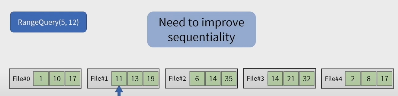
对于范围查询,将它分为多个 subrange。每个 subrange 包含指定数量的 key。
we keep track of the number of unique files accessed. Once the range query operation is done, we find the sub-range with the maximum number of unique files. If the number of unique files is larger than the threshold, called the sequentiality degree threshold, we add those unique files to the compaction candidate list.
This feature is useful in improving sequentiality especially for requests with Zipfian distribution (like YCSB [17]) where some keys are more frequently read and scanned.